Algorithms

An algorithm is a well-defined computational procedure that takes in a set of values as inputs and produces a set of values as outputs. An algorithm is thus a sequence of computational steps that transform input into output.

Nondecreasing order = an ordering where the next value is greater than or equal to the previous. Ex.
For values $x(n)$ and $x(n+1),\ x(n+1)>=x(n)$

Instance = an instance is a set of inputs to an algorithm that satisfy the input the input requirements.

Correct = an algorithm is said to be correct if, for every input instance, the computation halts when the correct output has been calculated.

Convex Hull = the smallest convex polygon that contains all points in a set of numbers that lie on a plane.

NP-complete problem = a problem for which there is currently no efficient algorithm that solves it, neither is there a proof that proves that the algorithm exists.

To prove an algorithm works, one way is by induction.

Start with the loop invariant, which is the subset of the input that is acted upon by the algorithm.

Then check for correctness in each of the following parts of the algorithm:

Initialization - Is it true prior to the first iteration of the loop?
Maintenance - Is it true at the start of the loop and also true at the end of the loop?
Termination - Is it true at the end of the loop?

Analyzing an algorithm is predicting how much resources it will use. You have to model the implemented technology.

Input size - A measure of the input must be selected that has the most significant impact on the resources required for an operation. For instance in a multiplication algorithm the input size should be number of bits used in the input numbers.

Running time - This should be a machine independent number. Number of primitive steps executed.

An algorithm's running time is dependent on the input data and there will be a best case, average case and worst case running time. The average case is often roughly as bad as the worst case. For instance with insertion sort.

Order of growth if the rate of growth of the running time. We consider the leading, most significant term of the formula of the worst case running time, called theta notation.

For an algorithm with a running time of $an^2 + bn + c$ the theta notation would be $Θ(n^2)$

Here's a breakdown of different sorting algorithms. There's sorting algorithms that sort in place, rely on element comparisons, others that don't.

For an unsorted list A of n length, loop through a growing subset of A by comparing the last element of the subset with each previous element and compare. If greater/smaller swap elements and iterate through again through a subset that is 1 larger than the previous.

1. for j = 1 to n
2.     key = A[j]
3.     i = j-1;
4.     while i > 0 and key < A[i]
5.        A[i+1] = A[i]
6.        i--
7.     A[i+1] = key

Find the smaller number and place it in A[1]. Then find smallest number in A[2..n] and place it in A[2]. Repeat

1. for i = 1 to A.length-1
2. 	//find the smallest number in A(i to n)
3. 	cur_smallest_index = i
4.	for j = i+1 to A.length
5.		if A[j] < A[cur_smallest_index]
6.			cur_smallest_index = j
7.	A[i] = temp
8.	A[i] = A[cur_smallest)index]
9.	A[cur_smallest_index] = temp;

Merge sort is an O(n lg n) sorting algorithm that uses the dive and conquer paradigm.

Heap sort is an O(n lg n) sorting algorithm that sorts in place with a constant number of array elements stored outside the array at any time.

Heapsort uses a data structure called a “heap” to manage information.

A heap is a binary-tree that consists of a root, and parent nodes that have up to two child nodes. The math to retreive the the parent, left element or right element of a node is really simple.

Parent - $return\lfloor i/2 \rfloor$
Left - $return 2*i$
Right - $return 2*i+1$

There are two kinds of binary heaps, max-heaps and min-heaps. In both kinds the values in the nodes satisfy a heap property. In max-heap the max-heap property is that for every node $i$ other than the root,

$A[Parent(i)]\geq A[i]$

For min-heap the min-heap property is that for every node $i$ other than the root,

$A[Parent(i)]\leq A[i]$

There are a set of operation algorithms that are used in conjuction with heaps. They are as follows:

• Max-Heapify
• Build-Max-Heap
• Heapsort
• Max-Heap-Insert, Heap-Extract-Max, Heap-Increase-Key, Heap-Maximum

Runs in O(lg n), whose inputs are A and index i into the array. When it is called, Max-Heapify assumes that the binary trees rooted at Left(i) and Right(i) are max-heaps, but that A[i] might be smaller than its children. Max-Heapify lets the A[i] value “float” down so that the subtree rooted at index i obeys the max-heap property.

1. Is index left smaller than A.heap-size and A[l] > A[i]?
   1. If yes, largest = l
2. Else, largest = i
3. Is index right smaller than A.heap-size and A[r] > A[i]?
   1. If yes, largest = r
4. Else, largest = i
5. If largest != i
   1. exchange A[i] with A[largest]
   2. Max-Heapify(A, largest)

Runs in $O(lg\ n)$ time.

Max-Heap Insert. Input: heap array A, with data from 1 to length, element to insert p
   // stuff the element at the end of the heap array
1. A[length+1] = p
   // iterate up through the heap
2. int i = length + 1;
3. while i >= 0
   // check if the parent node of our inserted element is less than it. 
4.    if (i/2 < p)
        // swap the inserted element with its parent
5.      A[i] = A[i/2]
6.      A[i/2] = p
7.      i = i/2
8.    else
9.      break

Build-Max-Heap uses Max-Heapify to a bottom-up manner to convert an array A[1..n], where n = A.length, in a max-heap. This procedure goes through the non-leaf nodes of the tree ($A[\lfloor n/2\rfloor..1]$) and runs Max-Heapify on each one.

Build-Max-Heap(A)
1. A.heap-size = A.length
2. for i = [A.length/2] down to 1
3.  Max-Heapify(A,i)

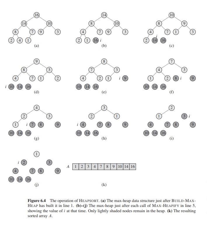
Heapsort works by building a max heap and then deconstructing it in order which in turn constructs a sorted array! Super neat and works in O(n lg n) time.

The algorithm works as follows:

Heapsort(A)

1. Build-Max-Heap(A)
2. for i = A.length down to 2 
3.  Exchange A[1] with A[i]
4.  A.heap-length -- 
5.  Max-Heapify(A)

Quick sort selects a random location within the array called a pivot.

Then it creates two lists, one containing all elements smaller than the pivot, and one containing all elements greater than the pivot.

Then it recursively calls its with each of those two new lists. When the lists end up being only one element long, it all gets merged.

Apparently heapsort is great and all, but quicksort beats it. What people do use is the heap data structure, with its most popular application being a priority queue. A priority queue is a data structure that contains a set of keys sorted by their priority. We use the following procedures when utilizing priority queues.

• Insert
• Find-Max

There are others that you can implement, but will make it difficult to address a element within the queue¹⁾.

• Delete-Max
• Change-Key

https://leetcode.com/explore/learn/card/recursion-ii/470/divide-and-conquer/2897/

Many algorithms are recursive, they call themselves recursively to deal with closely related sub-problems.

Divide - divide the problem into smaller subsets of the big set

Conquer - conquer the subproblems

Combine - combine the solutions to come up with the main solution of the bigger problem

A recurrence is an equation or inequality that describes a function in terms of its value of smaller inputs.

Methods for solving recurrences:

• substitution method guess a bound and then use mathematical induction to prove our guess correct
• recursion-tree method convert the recurrance into a tree whose nodes represent the costs incurred at various levels of the recursion.
• master method provides bounds for recurrences of the form $T(n) = aT(n/b) + f(n)$ where $a \geq 1,\ b\ > \ 1$ and $f(n)$ is a given function.

Validating a binary search tree can be solved with a divide and conquer approach. We check each node against an upper and lower bound. We then recurs and check both children.

Good video here.

The maximum subarray problem can be solved using divide and conquer.

By breaking up the input array into two subarrays of $n/2$ length as follows:

• A[low..mid]
• A[mid+1..high]

The maximum subarray A[i..j] can only be located in one of 3 places; in the first one, crossing the middle, or the end. To solve this equation we must find the maximum subarray in each of those 3 places and simply pick the biggest one.

Theres lots of little details in the maxCross function. Especially with dealing with finding the maximum of the subarrays when you have negative numbers. Where you start on the mid line counts. You had to go mid to left and mid+1 to the right. if you go mid-1 to the left you're screwed.

Find-Max-Crossing-Subarray Algorithm

int maxCross(vector<int>&nums, int& l, int &mid, int& r)
{
    // We don't have to do bounds checks because we know l won't equal r, 
    // because that's check for in the caller function.
    // With that knowledge we can set max_l and max_r both to INT_MIN's cause
    // I know there is going to be at least one element in each. You can also 
    // set to nums[mid] and nums[mid+1]
    int max_l = INT_MIN, max_r = INT_MIN;
 
    // find max left
    int sum = 0;
    for(int left = mid; left >= l; left-- )
    {
        sum += nums[left];
        max_l = max(sum, max_l);
    }
    // find max right
    sum = 0;
    for(int right = mid+1; right <= r; right++ )
    {
        sum += nums[right];
        max_r = max(sum, max_r);
    }
    // return the added sum.
    return max_l + max_r;
}
 
int maxSub(vector<int>& nums, int l, int r)
{
    if(l == r)
        return nums[l];
    int mid = (l+r) / 2; 
    int max_left  = maxSub(nums, l, mid);
    int max_right = maxSub(nums, mid + 1, r);
    int max_cross = maxCross(nums, l, mid, r);
    return max(max_left, max(max_right, max_cross) );
}
 
int maxSubArray(vector<int>& nums) {
    if(nums.size() == 0) return NULL;
    return maxSub(nums, 0, nums.size()-1);
}

This problem can also be solved very easily with a greedy version. Maximum Subarray Greedy

A greedy algorithm is used to find optimal soltions - minimum or maximums. Problems are solved in stages, with each stage choosing the optimal solutions. If a solution is found, add it to your solutions.

n = 5

a = { a₁, a₂, a₃, a₄, a₅ }

1. Algorithm Greedy(a,n)
2. for i=1 to n do:
3.    x = Select(a)
4.    if Feasible(x) Then:
5.        Solution = Solution + x

This problem can be solved amazingly easily in a one pass greedy approach. You keep track of a local maximum that can reset, and a global maximum.

int maxSubArray(vector<int>& nums) {
    int cur_max = nums[0], max_out = nums[0];
 
    for(int i = 1; i < nums.size(); i++)
    {
        cur_max = max(nums[i], cur_max + nums[i]);
        max_out = max(cur_max, max_out);
    }
    return max_out;
}

An approach for scanning through data is to use a sliding window technique.

For example, take this problem: find the length of the longest substring without repeating characters. Ex. Input: “abcabcbb” output = 3 (abc) and for “vadva” output = 3 (vadv)

To do this we have to scan through the input string while keeping track of the characters used. One such answer is as the following:

${\rm L{\small ONGEST}-S{\small UBSTRING}} (string)$

   // our sliding window will be bound by i and j
1. int i = 0; j = 0; max = 0
   // this is our hash table that contains a flag for every character
2. bool characterArray[128] = {false}
   // iterate up starting from i = 0
3. for int j from 0 to < string.length
       // if we've never seen this character before
       // and tally our max and update our character hash key  
4.     if characterArray(string[j]) = false 
5.         max = (max > (j+1-i)) ? max : (j+1-i)
6.         characterArray(string[j]] =  true)
       // if we have seen it before, reset it, and slide i forward one
       // and try again
7.     else
8.         characterArray(string[i]] = false)
9.         i++, j--
10. return max

Asymptotic efficiency is when we use an input size large enough to make only the growth of the running time relevant.

Worst case running time of an algorithm.

$$Θ(g(n)) = \{f(n)\ :\ there\ exist\ positive\ constants\ c_1,\ c_2,\ and\ n_0\ such\ that\\\ 0 \le c_1*g(n)\le f(n) \le c_2*g(n)\ for\ all\ n\ \ge\ n_0\}$$

O(g(n)) is defined as the set of functions which grow no faster than g(n).

$$0(g(n))\ =\ \{ f(n)\ :\ there\ exist\ positive\ constants\ c\ and\ n_0\ such\ that\\\ 0\leq f(n) \leq c*g(n)\ for\ all\ n\geq n_0\}.$$

or

$O(g(n))={f(n)\ :\exists\ c>0,\ n_0>0 \ni 0\leq f(n) \leq\ c*g(n) \forall n\geq n_0}$

Example²⁾:

Using this example of $f(n)=5n$ and $g(n)=n$ we can prove that $O(g(n))=n$.

The definition of $O(g(n))$ is:

$f(n)\in O(g(n))\iff \exists c>0,n_0\ni \forall n \geq n_0,f(n)\leq c*g(n) $

Using this definition we can prove that $f(n)$ is a member of $O(g(n))$:

$n\in O(g(n)) \iff \exists c>0, 5n \leq c*n $

By substituting constant c = 6:

$n\in O(g(n)) \iff \exists 6>0, 5n \leq 6*n$

Ω notation provides an asymptotic lower bound. For a given function $g(n)$, we denote by $Ω(g(n)$ (pronounced “big-omega of g of n” or “omega of g of n”) the set of functions

$$Ω(g(n))=\{f(n)\ :\ there\ exist\ positive\ constants\ c\ and\ n_0\ such\ that\\\ 0\leq c*g(n)\leq f(n)\ for\ all\ n\geq n_0\}$$.

We use o-notation to denote an upper bound that is not asymptotically tight. We define $o(g(n))$ as the set:

$$o(g(n)) = \{f(n)\ :\ for\ any\ positive\ constant\ c>0,\ there\ exists\ a\ constant\\\ n_0>0\ such\ that\ 0\leq f(n)\ < c*g(n)\ for\ all\ n \geq n_0\}.$$

Backtracking is an algorithm that looks at all possible solutions for a problem and evaluates each one.